Project 2: Fun with Filters and Frequencies

Tyler Yang

Overview

In this project, I explore the intricacies of utilizing low and high frequency filters to create some really neat images, blending multiple images seamlessly and create hybrid images in which depending on how far you are from the image, you ought to see two seperate images!

Part 1: Fun with Filters

Consider the partial derivatives for x and y. Utilizing the limit definition of a derivative, we can see that taking a partial derivative is the same as convolving with the differential operators below.

Figure 1: Notice that if we set x = x - 1 and h = 1, it is the exact same as convolving a matrix with the differential operators on the right!

To show the effects of the differential operator, we will use the cameraman image and apply the partial differential operators on the images. We see that we will get the result:

To calculate the gradient magnitude we simply take the square root of the sum of the squares of the partial derivatives. The formula for this is

As mentioned in my project 1, utilizing the gradient magnitude is a fantastic way to perform edge detection. Edges are areas of heavy intensity change, and the gradient magnitude measures this intensity change well! To show how this is so powerful, we can also binarize the gradient_magnitude image to show edges. To omit the noise, I chose the filter strength of 20% * the max gradient magnitude as the cutoff. Anything above 20% would be binarized to 1 and less to 0.

Smoothing The Image:

To smooth the image, we can utilize the Gaussian filter. We utilize cv.getGaussianKernel to create a 1D gaussian curve. Then, we can take the outer product of our 1D filter with its own transpose to achieve a 2D filter. We utilize a kernal_size of sigma * 6 with sigma = 5.

Image pulled from cv2 documentation of getGaussianKernel.

The left is a visualization of the 2d gaussian filter with kernal size sigma * 6 and sigma = 5. The right is the cameraman convolved with the gaussian filter.

The Gaussian filter does indeed reduce the noise in the image, however it also makes the edges less sharp. This results in far wider edges through the gaussian magnitude. In addition, some of the town in the back begin to become more noticeable due to gaussian smoothing.

On paper, because we are utilizing convolutions, we should be able to create a derivative of a Gaussian filter (DoG) first and then convolve this new filter with the cameraman to create the exact same gradient magnitude and binary edge image. You can see what the DoG filters visualized below:

The results of convolving the dOg filter with the cameraman image are shown below:

Practically, it is clear there are minute differences to the filtered images between our first method and this method. I suspect this has to do with some border artifacts and the way that he handle convolving the image with the filter. For these specific images - I made sure that both dx and dy convolutions were the same dimension through utilizing mode = valid and then cropping edges rather than using mode = same which means no edge padding. However, the results are still very similar to eachother verifying the commutative and associative properties of convolutions.

Part 2: Fun with Frequencies

Sharpening

We utilize an unsharp masking technique for our image filter in order to sharpen an image. In essense, to sharpen an image, we want to add our high frequency values back to the original image so the edges are more pronounced. Since we already calculated a low-frequency filter in the previous section, we can subtract an image by its gaussian smoothed version to optain the high frequencies.

However, we want to make a filter that performs all these intermediate steps before hand so we can do one convolution and optain a sharper image. This is our unsharp mask filter.

If a is a hyper parameter that defines how much to add our high-frequencies back to the original image, we can derive a new filter that is our unit impulse - our low-frequency gaussian filter.

An interesting observation would be to take a sharpened image, blur it and then use our unsharp technique to try to sharpen it again. I have decided to use my headshot for this. The results are below:

Clearly, sharpening our blurred image will not produce the same results as our original sharpened image. This is because when we blur our image the first time, we already remove alot of the higher frequencies. We are simply adding higher frequencies of the smoothed image. However, we can notice that our sharpened image is still sharper than our blurred image.

Hybrid Images

With our low and high frequency filters, we can do something really cool - we can overlap the low frequencies of one image with the high frequencies of another image and create a hybrid image, in other words depending on resolution you will see two seperate images! For each image, I utilized seperate sigma values for the low and high frequency filters to obtain the best results.

Nutmeg the cat is high frequency while Derek is low frequency. This means that you should be able to see derek if you lower the resolution or look at it from afar while nutmeg should be prominent close up.

To the left, the high frequencies of Brown Teddy Junior (Btjr) are combined with the low frequencies of arctic. They form the amalgamation that is to the right.

However, sometimes we cannot really blend our hybrid images with our current method.

No matter what sigmas we set for the low and high frequency filters, we cannot seem to get the white pants to shine through. This is because the contrast between the white and black pants are too high and the low frequencies of the black pants will always dominate the high frequencies of the white pants.

We can also see this effect in the frequency basis. In my example below (where I am flexing and standing in the Astor Plaza subway station of New York City), we can transform each one of these images to the frequency basis by performing a fourier transform. The most prominent frequencies are horizontal and vertically due to the amount of grids and lines in the subway station. When we apply our low-frequency filter we can clearly see that the spikes of the frequencies are more condensed towards the center or in other words less intense. Utilizing the unsharp mask filter, we can see that in the frequency basis, the spikes are augmented showing more intense frequencies all around.

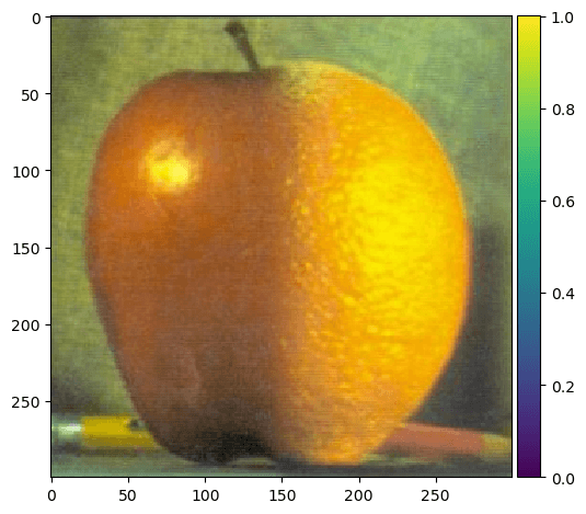
Oraple

We can take our low-frequency and high-frequency filters even farther. Consider an image of an Apple of an Orange. If we were to splice these two images together we would get half an apple and half an orange. The edge difference is clear. What if there was a way to seemlessly blend these two fruits.

How do we go about blending these two images? We can utilize gaussian and laplacian stacks. A gaussian stack is simply convolving the gaussian filter over and over again so the image becomes smoother and smoother (lower frequencied). Then, we can conversly create our laplacian stack from our gaussian stack by subtracting the difference of the n+1 layer of the gaussian stack with the nth layer of the gaussian stack. This will give us a stack of higher and higher frequencies until we reach the original image.

To create our blended image, we follow the process outlined in Burt and Adelson 1983. First, we build the Laplacian Stacks for our two images (one for apple and one for orange). Then, we build a Gaussian stack out of our mask (in this case we are utilizing a binary mask, meaning that everything past the horizontal halfwaypoint will be 1 and before will be 0). We then can form a combined pyramid utilizing our mask gaussian stack as weights. The official calculation would be LS_l = LA_l * GR_l + (1 - GR_l) * LB_l. The final step is to sum all the levels of our stack to form our final image.

Figure: Oraple Stack - the left column is the masked apple stack, the middle is the masked orange stack, and the end is the combined stack. Each row represents a higher level in the combined laplacian stack. (the top row is the 0th layer, the second to last is the 5th layer, while the bottom is combining the stack.). In order to make the first few layers visible, I needed to normalize the images to a range of 0-1. As a Note, the last layer (second to last row ) is actually the final layer of the gaussian stacks of the original images. This is necessary to form the final image as it adds the final lowest frequencies that we would infinitely approach the more laplacian stack layers we have.

Our oraple is complete on the bottom right hand corner of the image - and it is impressive!

Lets explore this with some other images. Our first image is combining a Boeing 747 with a fighter jet. Practically this would never exist due to differing functionalities but it would be cool. I decided to use a United liveried 747-400. Below is the result of the blending.

Hmm, the Oraple was definitely more impressive. The main problem with this blending are the colors are simply too distinct from eachother and with only 5 layers of the laplacian pyramid, its hard to completely seamlessly blend the jarring color change. Lets try an old KLM boeing 747.

We can also create an irregular mask! Since it was the autumn equinox recently, I decided to celerate fall by utilizing a pumpkin photo. Can you find the imposter pumpkin! The mask is actually an ellipse image read in to which I simply binarized the image. The mask and image alignments were performed in Figma.